data mining, forward + backward + ridge + lasso + pcr + pls

linear model

Y=β_0+β_1 X_1+…+β_p X_p+ϵ (Least squares methods)

Forward Stepwise Selection

- Best subset selection은 2^p개의 model을 고려해야하므로 p가 크면 사용하기 힘듦

- Null model에서 시작하여 한번에 한 개씩의 explanatory variable을 추가함

Backward Stepwise Selection

- Full model에서 시작하여 한번에 한 개씩의 explanatory variable을 제외함

 

To choose a model with a low test error

1. estimate test error indirectly by making an adjustment to the training error

 ex) C_p, AIC, BIC and adjusted R^2 

2. estimate the test error directly using CV approach

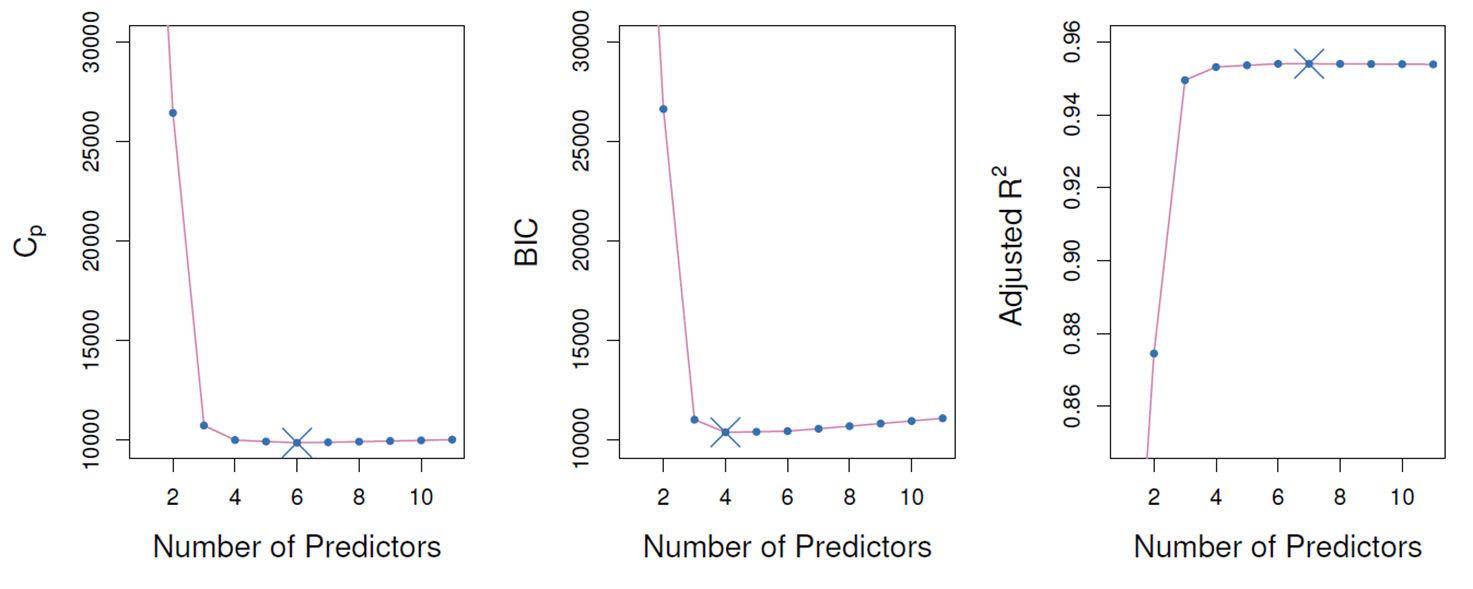
- C_p=1/n(RSS+2kσ ̂^2) where RSS: RSS on a training data

- AIC=-2lnL ̂+2k=nln(RSS/n)+2k where L ̂: maximum value of the likelihood

 - BIC=-2lnL ̂+kln(n)=nln(RSS/n)+kln(n)

(변수 개수가 많은 model에 더 심한 penalty를 부여하여 AIC보다 더 작은 크기의 model선택)

- Adjusted R^2=1-(RSS/(n-k-1))/(TSS/(n-1))  (R^2=1-RSS/TSS)

(변수가 많아 지면서 RSS가 감소하므로 더 작은 값으로 나누어 R^2 값을 감소시킴)

K-fold CV

- In the past, with large p and/or large n,

 

- C_p, AIC, BIC, and adjusted R^2 were more attractive approaches for choosing among a set of models

 

-  K-fold CV is a very attractive approach for choosing among a set of models

Ridge regrssion

- ridge regression coefficient estimates β ̂^R

- β_j (j=1,…,p)의 제곱 합으로 penalty를 주기 때문에 전체적으로 β_j를 수축 (shrinkage)시키는 효과가 발생 (intercept β_0는 제외)

- tuning parameter λ(≥0) 가 0일 때는 ridge regression coefficient는 least squares estimate과 같게 되지만 λ→∞에 따라 coefficient는 0으로 수렴하게 됨

- tuning parameter λ는 k-fold CV로 결정

- Least squares estimates은 explanatory variable 의 scale에 영향을 받지 않지만 ridge regression coefficient는 penalty term때문에 explanatory variable의 scale의 크게 의존

- Ridge regression fitting전에 explanatory variable을 standardization할 필요가 있음 (SE로 나누어 줌)

Lasso regrssion

- lasso coefficient estimates β ̂^L

- ridge regression의 단점은 β_j 의 값을 수축시키지만 정확하게 0을 만들지 못한다는 점인데 lasso는 coefficient estimates을 0으로 수축시킴

- tuning parameter λ(≥0) 가 0일 때는 lasso coefficient는 least squares estimate과 같지만 λ가 충분히 크게 되면 모든 coefficient가 0인 null model이 됨

- tuning parameter λ는 k-fold CV로 결정

- Lasso fitting전에 explanatory variable을 standardization할 필요가 있음

PCA

- n × p data matrix X의 dimension을 줄이는 기법

- First PC (PC1): direction of largest sample variance

- Z_1=0.839∗(pop-(pop) ̅ )+0.544∗(ad-(ad) ̅)

- Second PC (PC2) : (1) orthogonal to PC1 (2) again largest sample variance

- Z_1=0.544∗(pop-(pop) ̅ )-0.839∗(ad-(ad) ̅)

- Third PC (PC3) : (1) orthogonal to PC1, PC2 (2) again largest sample variance etc.

- First M principal components, Z_1, . . ., Z_M  as the predictors in a linear regression model that is fit using least squares

- X_1, . . ., X_p의 변동이 큰 방향들이 Y와 관련이 있는 방향이라 가정한다면 least squares을 Z_1, . . ., Z_M에 적합하는 것이 X_1, . . ., X_p에 적합하는 것 보다 더 나을 수 있음

- Most of the information in the data that relates to the response is contained in Z_1, . . ., Z_M, and by estimating only M (<p) coefficients we can mitigate overfitting

- Number of principal components, M, is typically chosen by k-fold CV

- Recommend standardizing each predictor

PLS

- PCR approach involves identifying linear combinations, or directions, that best represent the predictors X_1, . . .,X_p  in an unsupervised way

- PLS (partial least squares) is a supervised alternative to PCR (i.e. response variable Y를 이용하여 X_1, . . .,X_p를 잘 근사할 뿐만 아니라 Y와 관련된 새로운 변수를 생성)

First PLS direction: compute Z_1 by setting each ϕ_j1 equal to the coefficient from the simple linear regression of Y onto X_j à Z_1=∑2_(j=1)^p▒〖ϕ_j1 X_j 〗 (i.e. response variable Y와 가장 강하게 관련 있는 X_j에 가장 높은 가중치를 부여)

- Second PLS direction: take residuals by regressing each variable on Z_1 and then compute  Z_2 using this orthogonalized data in the same as Z_1 was computed based on the original data (X_j의 residuals은 Z_1에 의해 설명되지 않고 남아 있는 정보로 해석 가능)

- Repeated M times to identify multiple PLS components Z_1, . . ., Z_M

- Number M of partial least squares directions used in PLS is a tuning parameter that is typically chosen by k-fold CV

- standardize the predictors and response before performing PLS

 

#Best subset selection
library(ISLR)
head(Hitters)
dim(Hitters)
sum(is.na(Hitters))
Hitters <- na.omit(Hitters)
dim(Hitters)
library(leaps)
regfit.null <- regsubsets(Salary ~., Hitters)
summary(regfit.null) #변수 총 19개 CRBI가 첫번째 BEST, 두 번째 HIT, ... 8variable/ best만을 뽑는 방법

regfit.null <- regsubsets(Salary ~., Hitters, nvmax = 10)
res <- summary(regfit.null)
names(res)
res$rsq #r square
res$bic # 적을수록 좋음 
plot(res$rss, xlab = "# of variables", ylab = "RSS", type = "l")
plot(res$adjr2, xlab = "# of variables", ylab = "adj2", type = "l") # 변수 penalty , 어느정도 되면 줄어든다 
which.max(res$adjr2)
points(10,res$adjr2[10], col = "red", cex= 2,pch =20)

#forward and backward stepwise selection 
regfit.fw <- regsubsets(Salary ~., Hitters, nvmax = 19, method = "forward")
summary(regfit.fw)

regfit.bw <- regsubsets(Salary ~., Hitters, nvmax = 19, method = "backward")
summary(regfit.bw)

coef(regfit.null, 7)
coef(regfit.fw, 7)
coef(regfit.bw, 7)

# (3) model selection using validation set approach
set.seed(1)
train <- sort(sample(1:nrow(Hitters), 132))
test <- setdiff(1:nrow(Hitters), train)
regfit.best <- regsubsets(Salary~., Hitters[train,], nvmax=19)
test.mat <- model.matrix(Salary~., Hitters[test,])
dim(test.mat)
head(test.mat)
val.error <- rep(NA, 19)
for(i in 1:19){
  coefi <- coef(regfit.best, id = i)
  pred <- test.mat[, names(coefi)] %*% coefi
  val.error[i] <- mean((Hitters$Salary[test]-pred)^2)
}
val.error 
which.min(val.error)

regfit.best <- regsubsets(Salary~., Hitters, nvmax= 19)
coef(regfit.best, id = 6) # 이게베스트

# (4) model selection using K-fold CV
k <-10
set.seed(1)
folds <- sample(1:k, nrow(Hitters), replace = T)
table(folds)
263/10
cv.errors <- matrix(NA, k, 19, dimnames = list(NULL, paste(1:19)))
cv.errors
j=1
i=1
for(j in 1:k) {
  best.fit <- regsubsets(Salary~., data = Hitters[folds!=j,], nvmax = 19)
  test.mat <- model.matrix(Salary~., Hitters[folds==j,])
  for(i in 1:19){
    coefi <- coef(best.fit, id = i)
    pred <- test.mat[, names(coefi)] %*% coefi
    cv.errors[j, i] <- mean((Hitters$Salary[folds==j]- pred)^2)
  }
}
mean.cv.errors <- apply(cv.errors, 2, mean)
mean.cv.errors
plot(mean.cv.errors, type = "b")
which.min(mean.cv.errors)

reg.best <- regsubsets(Salary~., Hitters, nvmax = 19)
coef(reg.best, id =10)

#(5) ridge regression
library(glmnet)
x <- model.matrix(Salary~., Hitters)[,-1]
y <- Hitters$Salary
ridge.mod <- glmnet(x, y, alpha = 0, lambda = 10^seq(10, -2, length=100)) # 알파가 0이면 ridge, 1이면 lasso 
coef(ridge.mod)
ridge.mod$lambda[50]
coef(ridge.mod)[,50]

set.seed(1)
dim(Hitters)
train <- sort(sample(1:nrow(Hitters), 132))
test <- setdiff(1:nrow(Hitters), train)

y.test <- y[test]
ridge.mod <- glmnet(x[train, ],y[train], alpha = 0, lambda = 10^seq(10, -2, length = 100))
ridge.pred <- predict(ridge.mod,s =4,newx =x[test,])
mean((ridge.pred - y.test)^2)

[1] 139839.6

# select the best lambda using k-fold CV
set.seed(1)
cv.out <- cv.glmnet(x[train,], y[train], alpha=0)
plot(cv.out)
best.lambda <- cv.out$lambda.min
best.lambda
ridge.pred <- predict(ridge.mod, s = best.lambda, newx = x[test,])
mean((ridge.pred-y.test)^2)

out <- glmnet(x, y, alpha = 0)
predict(out, type = "coefficients", s = best.lambda)

#(6) lasso
lasso.mod <- glmnet(x[train,], y[train], alpha = 1, lambda = 10^seq(10, -2, length = 100))
plot(lasso.mod)

set.seed(1)
cv.out <- cv.glmnet(x[train,], y[train], alpha = 1)
plot(cv.out)

best.lambda = cv.out$lambda.min
best.lambda
log(best.lambda)
lasso.pred <- predict(lasso.mod, s = best.lambda, newx = x[test,])
mean((lasso.pred-y[test])^2)

out <- glmnet(x, y, alpha = 1)
coef.lasso <- predict(out, type = "coefficients", s = best.lambda)
coef.lasso[coef.lasso != 0]

# (7) PCR
library(pls)
library(ISLR)
head(Hitters)
dim(Hitters)
sum(is.na(Hitters))
Hitters <- na.omit(Hitters)
dim(Hitters)

set.seed(1)
train <- sort(sample(1:nrow(Hitters), 132))
test <- setdiff(1:nrow(Hitters), train)

x <- model.matrix(Salary~., Hitters)[,-1]
y <- Hitters$Salary
y.test <- y[test]

#fit PCR with all data
set.seed(2)
pcr.fit <- pcr(Salary~., data = Hitters, scale = T, validation = "CV")
pcr.fit
summary(pcr.fit)
validationplot(pcr.fit, val.type = "MSEP") #MSEP : Prediction에 대한 MSE
#2~3개만 넣어도 상당히 정확하다고 볼 수 있음, 한개 component만 해도 40%정도 설명

#fit PCR with training/test data
set.seed(1)
pcr.fit <- pcr(Salary~., data = Hitters, subset = train, scale = T, validation = "CV")
validationplot(pcr.fit, val.type = "MSEP")

pcr.pred <- predict(pcr.fit, newdata = x[test,], ncomp = 5)
mean((pcr.pred-y.test)^2)

pcr.fit <- pcr(y~x, scale = T, ncomp = 5)
summary(pcr.fit)

#(8) partial least square(PLS) > 변수를 줄이기 위해 변수들 간의 relation이 높은 것 위주로 만드는 것 
library(pls)
pls.fit <- plsr(Salary~., data = Hitters, subset = train, scale = T, validation = "CV")
summary(pls.fit) # 감소했다가 증가했다가 
validationplot(pls.fit, val.type = "MSEP") #2개에서 거의 최소 
pls.pred <- predict(pls.fit, x[test,], ncomp = 3)
mean((pls.pred-y.test)^2)
pls.fit <- plsr(Salary~., data = Hitters, scale = T, ncomp = 3)
summary(pls.fit)

data mining, forward + backward + ridge + lasso + pcr + pls