통계 이야기
data mining, maximal margin classifier + support vector classifier + support vector machine in R
728x90
반응형
< Generalization of a simple and intuitive classifiers >
- Maximal margin classifier (최대 마진 분류기): linear boundary로 class 구별 (에러 없음)
- Support vector classifier (서포트 벡터 분류기): linear boundary & soft margin classifier (에러 포함)
- Support vector machines (서포트 벡터 머신): non-linear class boundaries
Maximal margin classifier (최대 마진 분류기)
- Separating Hyperplane (분리 초평면)
•Suppose a hyperplane that separates the training observations perfectly according to their class labels (p-dimension, n samples, p predictors)
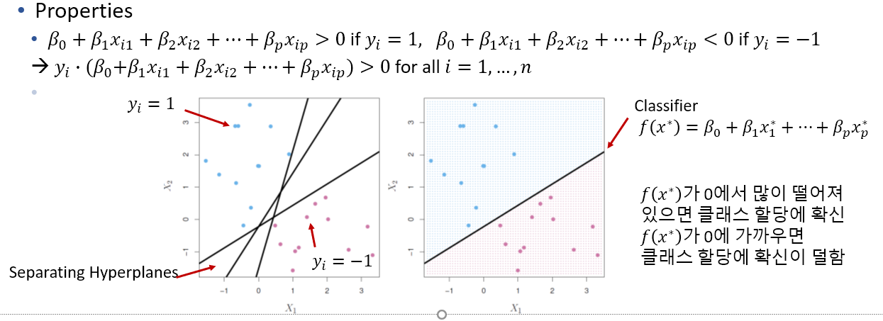
- margin: minimal distance from observations to hyperplane
- maximal margin hyperplane: separating hyperplane for which the margin is largest
- support vectors: maximal margin hyperplane depends directly on the support vectors, but not on the other observations
Support Vector Classifiers (서포트 벡터 분류기 )
- Greater robustness to individual observations
- Better classification of most of the training observations
- Called a soft margin classifier
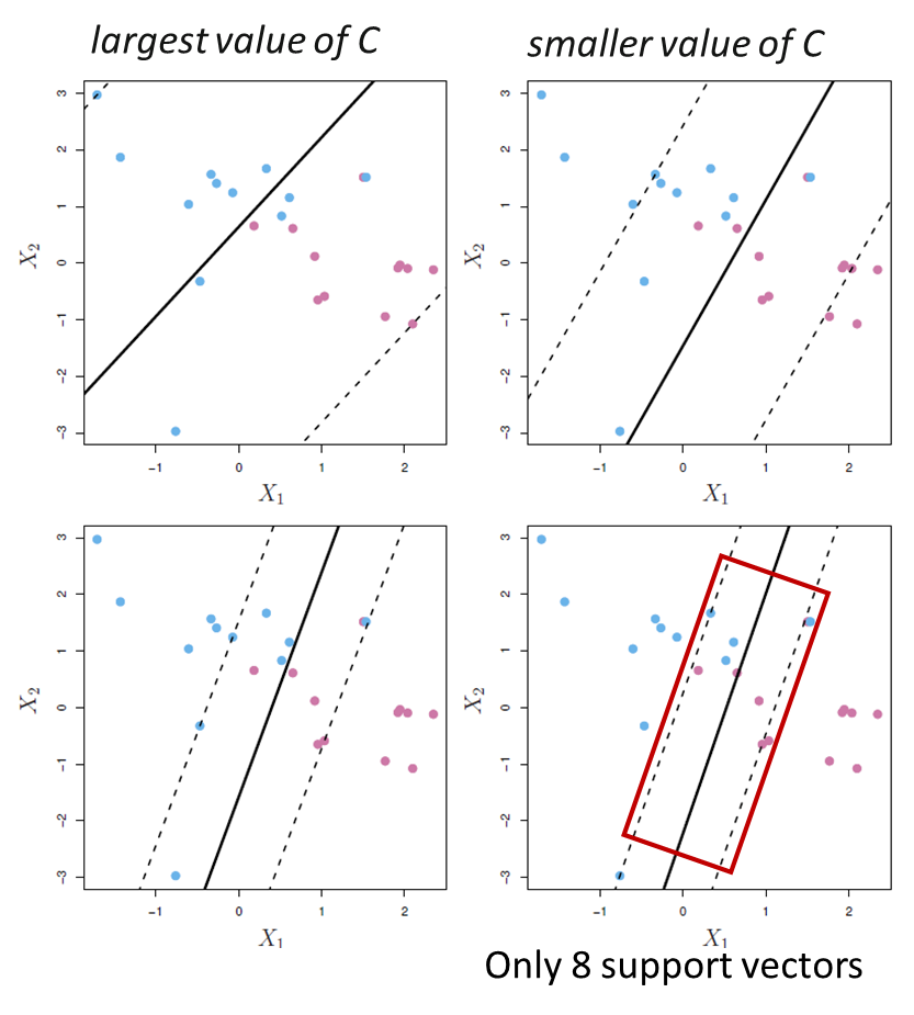
< K-fold CV for tuning parameter C >
- C is small: narrow margins, highly fit to the data, low bias but high variance
- C is larger: wider margins, fitting the data less, higher bias but lower variance
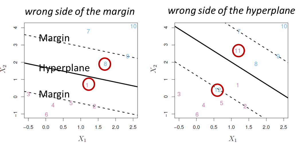
< Support vectors >
- margin상에 직접 놓이거나 margin을 위반한 관측치들
- Support vectors들만 classifier에 영향을 줌
- Support vectors 이외의 관측치들은 classifier 생성에 영향을 주지 않는 않는다는 점이 특징
Support Vector Machines (서포트 벡터 머신)
- Non-linear Decision Boundaries

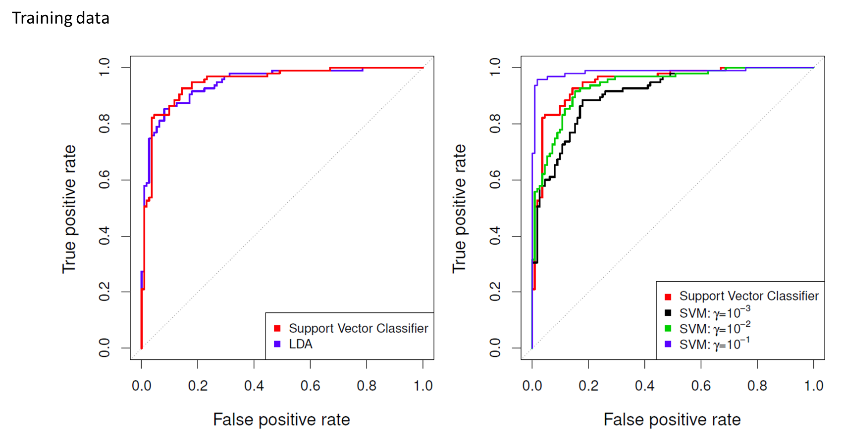
- address the problem of possibly non-linear boundaries between classes
< Generalized support vector classifier -> SVM >
- Kernel: generalization of the inner product (두 함수의 유사성을 수량 화하는 함수)

---------------코드
# support vector classifier
#시뮬레이션 데이터 생성
#training data 생성
set.seed(1)
x <- matrix(rnorm(20*2), ncol = 2)
y <- c(rep(-1, 10), rep(1, 10))
dim(x)
x
x[y == 1,] <- x[y == 1] + 1
plot(x, col =(3-y), pch = 16) #y = 1, 2 = "red" / y = -1, 4 = "blue"
dat <- data.frame(x =x , y = as.factor(y))
head(dat)
#test data 생성
xtest <- matrix(rnorm(20*2), ncol = 2)
ytest <- sample(c(-1, 1), 20, rep = T)
table(ytest)
xtest [ytest==1,] <- xtest[ytest==1,]+1
testdat <- data.frame(x=xtest, y=as.factor(ytest))
head(testdat)
#support vector classifier
install.packages("e1071")
library(e1071)
svmfit <- svm(y~., data = dat, kernel = "linear", cost = 10, scale = F)
plot(svmfit, dat)
names(svmfit)
svmfit$index # plot에서 support machine은 x로 표시된다
svmfit <- svm(y~., data = dat, kernel = "linear", cost = 0.1, scale = F)
plot(svmfit, dat) #cost가 작아지면 support vector가 많아진다. 이게 많아진다는 이야기는 margin이 넓어진다는 뜻. c가 작아지면 margin이 커진다.
svmfit #cost는 10-ford crossvalidation으로 결정


#10-fold CV
set.seed(1)
tune.out <- tune(svm, y~., data = dat, kernel = "linear", ranges = list(cost = c(0.001, 0.01, 0.1, 1, 5, 10, 100)))
tune.out
summary(tune.out)
bestmd  <- tune.out$best.model
bestmd

ypred <- predict(bestmd, newdata = testdat)
table(ypred, testdat$y)
# support vector machine (non-linear)
#generate data
set.seed(1)
x <- matrix(rnorm(200*2), ncol = 2)
x[1:100,] <- x[1:100,]+2
x[101:150,] <- x[101:150,] -2
y <- c(rep(1, 150), rep(2,50))
dat <- data.frame(x=x,y=as.factor(y))
plot(x,col = y+1,pch = 16) #y=1 -> col = 2 . y=2 ->col=3
#fit SVM with radial kernel
train <-sort(sample(200, 100))
test<-setdiff(1:200, train)
svmfit <- svm(y~., data = dat[train,], kernel = "radial", gamma = 1, cost = 1)
summary(svmfit)
plot(svmfit,data = dat[train,])
svmfit <- svm(y~., data = dat[train,], kernel = "radial", gamma = 1, cost = 1e5)
summary(svmfit)
plot(svmfit,data = dat[train,])
svmfit <- svm(y~., data = dat[train,], kernel = "radial", gamma = 2, cost = 1)
summary(svmfit)
plot(svmfit,data = dat[train,])
#10-fold CV
set.seed(1)
tune.out <- tune(svm, y~., data = dat[train,], kernel = "radial", ranges = list(cost = c(0.1, 1, 10, 100, 1000), gamma = c(0.5, 1, 2, 3, 4, 5)))
tune.out
summary(tune.out)
testy <- dat[test,]$y
predy <- predict(tune.out$best.model, newx = dat[test,])
table(testy, predy)


728x90
반응형
'통계 이야기' 카테고리의 다른 글
| data mining, polynomial regression + step functions + Natural cubic spline + smoothing spline + local regression + GAM in R (0) | 2021.12.18 |
|---|---|
| data mining, forward + backward + ridge + lasso + pcr + pls (0) | 2021.12.17 |
| data mining, random forest + boosting in R (0) | 2021.12.15 |
| Data Mining , Classification tree + Regression tree + Bagging (0) | 2021.12.14 |
| Simulation 공부 with R (0) | 2021.10.02 |
댓글