빅데이터 분석 ; LDA ; logistic regression ; dicision tree ; 동시 비교

Select Language English Japanese Korean
안녕하세요. 창이에요 !
kaggle data인 social_network_ads 데이터를 가지고 빅데이터 분석을 해보았습니다.
LDA, logistic regression, dicision tree를 각각 만들어보고
어떤 방법으로 반복, 시행 했을 때 가장 높은 평균과 표준편차를 갖는지 알아보겠습니다.
LDA
데이터 불러오기
data <- read.csv('Social\_Network\_Ads.csv')
head(data)
attach(data)

dim(data)
[1] 400 5
데이터셋 들여다보기
str(data)
결측치 확인
sum(is.na(data))[1] 0
plot 그리기 위한 4분할
par(mfrow= c(2, 2))
barplot(table(data$Gender))
barplot(table(data$Purchased))
hist(data$Age)
hist(data$EstimatedSalary)
summary(data)
seed 주기
set.seed(421)총 400개 데이터 중 70%를 train, 나머지를 test로 지정한다.
index <- sample(nrow(data),nrow(data)*0.7)
train<-data[index,]
test<-data[-index,]
for (x in list("Purchased")){
train[[x]]<-as.factor(as.character(train[[x]]))
test[[x]]<-as.factor(as.character(test[[x]]))
}
library(MASS)
ld1 <- lda(formula = Purchased~Gender + Age + EstimatedSalary, data = data)
ld1

pred1 <- predict(ld1,test)
y1 <- table(pred1$class,test$Purchased)
y1
0 1
0 71 15
1 5 29
정확도
accuracy<-function(x){
sum(x[row(x) == col(x)])/sum(x)
}
accuracy(y1)
[1] 0.8333333
오분류율
1-accuracy(y1)[1] 0.1666667
(여러 사전확률에 따른 모델의 성능 확인)
set.seed(NULL)
accuracy<-function(x){
sum(x[row(x) == col(x)])/sum(x)
}acc <- c()
for (x in 1:10){
index <- sample(nrow(data),nrow(data)*0.7)
train<-data[index,]
test<-data[-index,]
ld1 <- lda(formula = Purchased ~ Gender + Age + EstimatedSalary, data = train)
pred1 <- predict(ld1,test)
y1 <- table(pred1$class,test$Purchased)
acc<-c(acc,accuracy(y1))
}

acc
[1] 0.8416667 0.8333333 0.8333333 0.8833333 0.8750000 0.8250000 0.8166667 0.8333333 0.8833333 0.8500000
m <- mean(acc)
s <- sd(acc)

# 7:3의 확률일 때

acc1 <- c()
for (x in 1:10){
index <- sample(nrow(data),nrow(data)*0.7)
train<-data[index,]
test<-data[-index,]
ld1 <- lda(formula = Purchased ~ Gender + Age + EstimatedSalary, data = train,prior = c(0.7,0.3))
pred1 <- predict(ld1,test)
y1 <- table(pred1$class,test$Purchased)
acc1<-c(acc1,accuracy(y1))
}

acc1
[1] 0.8500000 0.8333333 0.7833333 0.8750000 0.8750000 0.8083333 0.8000000 0.7750000 0.8000000 0.7833333
m1 <- mean(acc1)
s1 <- sd(acc1)

# 3:7의 확률일 때

acc2 <- c()
for (x in 1:10){
index <- sample(nrow(data),nrow(data)*0.7)
train<-data[index,]
test<-data[-index,]
ld1 <- lda(formula = Purchased ~ Gender + Age + EstimatedSalary, data = train,prior = c(0.3,0.7))
pred1 <- predict(ld1,test)
y1 <- table(pred1$class,test$Purchased)
acc2<-c(acc2,accuracy(y1))
}

acc2
[1] 0.7916667 0.7750000 0.8166667 0.8166667 0.7833333 0.7916667 0.7583333 0.8416667 0.8083333 0.7083333
m2 <- mean(acc2)
s2 <- sd(acc2)

c(m, m1, m2)
[1] 0.8475000 0.8183333 0.7891667
c(s, s1, s2)[1] 0.02454839 0.03763863 0.03707059
boxplot으로 비교하기
boxplot(list(acc,acc1,acc2),names = c("default","7:3","3:7"),
main = "Accuracy Box-plot" )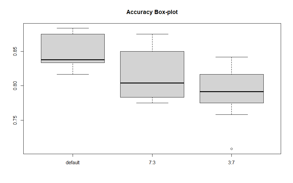

Logistic Regression
모형 적합
glm.obj <- glm(Purchased ~ Gender + Age + EstimatedSalary, data = data, family = binomial) ; summary(glm.obj)
Gender 변수의 P 값이 0.05보다 크므로 변수 제거.
glm.obj <- glm(Purchased ~ Age + EstimatedSalary, data = data, family = binomial) ; summary(glm.obj)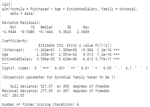
데이터 나눈 후 반복. 임계값 0.5
for (x in 1:10){
ind = sample(nrow(data1),nrow(data1)*0.7)
train = data1[ind,]
test = data1[-ind,]
glm = glm(Purchased ~ ., data=train,family=binomial())
pred_glm = predict(glm,test)
pred_glm[pred_glm > 0.5] = 1
pred_glm[pred_glm < 0.5] = 0
tab_glm = table(pred_glm,test$Purchased)
accu_glm = c(accu_glm,accuracy(tab_glm))
}

mean(accu_glm);sd(accu_glm)
[1] 0.8225
[1] 0.02779166
임계값 0.3 으로 10번 반복
accu_glm = c()
for (x in 1:10){
ind = sample(nrow(data1),nrow(data1)*0.7)
train = data1[ind,]
test = data1[-ind,]
glm = glm(Purchased ~ ., data=train,family=binomial())
pred_glm = predict(glm,test)
pred_glm\[pred_glm > 0.3] = 1
pred_glm[pred_glm < 0.7] = 0
tab_glm = table(pred_glm,test$Purchased)
accu_glm = c(accu_glm,accuracy(tab_glm))
}

mean(accu_glm);sd(accu_glm)
[1] 0.83
[1] 0.03689324
임계값 0.7로 반복
for (x in 1:10){
ind = sample(nrow(data1),nrow(data1)*0.7)
train = data1[ind,]
test = data1[-ind,]
glm = glm(Purchased ~ ., data=train,family=binomial())
pred_glm = predict(glm,test)
pred_glm[pred_glm > 0.7] = 1
pred_glm[pred_glm < 0.3] = 0
tab_glm = table(pred_glm,test$Purchased)
accu_glm = c(accu_glm,accuracy(tab_glm))
}

mean(accu_glm);sd(accu_glm)
\[1\] 0.7179167
\[1\] 0.121524
Dicision Tree
library(rpart)
library(rpart.plot)
test <- read.csv("Social_Network_Ads.csv")
test <- test[c(2:5)]

# 구매여부에 대한 분포와 entrophy

tar<-matrix(table(test$Purchased),nrow = 1)
tot<-sum(tar)
tar<-cbind(tar,tot)
colnames(tar) <- c("not buy","buy","total")
dist<-tar/tot
ent <- 0
for (x in 1:(ncol(dist)-1)){
ent <- sum(ent,-dist[x] * log(dist[x]))
}
not.buy buy total ent
1 257 143 400 0.6519662
tar<-data.frame(tar,ent)
tar
연속형 변수 범주화 및 기대 엔트로피와 정보이득 계산 함수
expect<-function(mat){
mat<-cbind(mat,rowsum=rowSums(mat))
mat<-rbind(mat,colsum=colSums(mat))
kk <- list()
for (x in 1:(nrow(mat)-1)){
kk[[x]] <- mat[x,] / mat[,ncol(mat)][[x]]
}

entro<-sapply(kk,function(x){
ent <- 0
for (i in 1:(length(x) - 1)){
ent <- sum(ent,-x[[i]] * log(x[[i]]))
}
ent
})
entro<-c(entro,tar$ent)
mat<-data.frame(mat,entropy=entro)
print(mat)
expect_ent<-sum(mat$entropy[1:length(mat$entropy)-1] * mat$rowsum[1:length(mat$rowsum)-1]/tot)
cat("\n기대 엔트로피:",expect_ent)
info<- tar$ent- expect_ent
cat("\n정보이득:",info)
}

    # age 변수 범주화 및 기대 엔트로피, 정보이득 구하기


age_Category<-cut(test$Age,c(0, 30, 60))
test$Age<-age_Category
mat<-table(test$Age,test$Purchased)
dimnames(mat) <- list("Age" = c("MZ세대", "babyboomer"),
"Purchased" = c("not buy","buy"))
not.buy buy rowsum entropy
MZ세대 105 6 111 0.2102834
babyboomer 152 137 289 0.6917996
colsum 257 143 400 0.6519662
expect(mat)기대 엔트로피: 0.5581789
정보이득: 0.09378734
salary 변수 범주화 및 기대 엔트로피와 정보이득 구하기
salary_category <- cut(test$EstimatedSalary, c(0, 50000, 100000, 1500000))
test$EstimatedSalary <- salary_category
mat <- table(test$EstimatedSalary, test$Purchased)
dimnames(mat) <- list( "Salary" = c("저소득", "중소득", "고소득"), "Purchased" = c("not buy", "buy"))
expect(mat)
not.buy buy rowsum entropy
저소득 80 44 124 0.6503906
중소득 166 37 203 0.4748122
고소득 11 62 73 0.4238953
colsum 257 143 400 0.6519662
기대 엔트로피: 0.5199492
정보이득: 0.1320
이산형 변수인 Gender 변수의 기대 엔트로피와 정보이득 구하기
mat <- table(test$Gender, test$Purchased)
dimnames(mat) <- list( "Sex" = c("male", "female"), "Purchased" = c("not buy", "buy"))
expect(mat)
not.buy buy rowsum entropy
male 127 77 204 0.6628025
female 130 66 196 0.6388458
colsum 257 143 400 0.6519662
기대 엔트로피: 0.6510637
정보이득: 0.0009024999
변수들 범주화
test$Purchased <- ifelse(test$Purchased ==1, '구매', '비구매')
test$Purchased <- as.factor(test$Purchased)
test$Gender <- as.factor(test$Gender)
test$Age <- ifelse(test$Age >= 10 & test$Age < 30, "MZ세대", 'babybomer')
test$Age <- as.factor(test$Age)
test$EstimatedSalary <- ifelse(test$EstimatedSalary > 10000 & test$EstimatedSalary <= 50000, "little",
ifelse(test$EstimatedSalary > 50000 & test$EstimatedSalary <= 100000, "middle", "much"))
test$EstimatedSalary <- as.factor(test$EstimatedSalary)
test <- test[c(2:5)]

# train : test = 7 : 3 / 20개 set으로 분리

train <- vector("list",10)
data <- vector("list",10)
for (x in 1:10){
index <- sample(nrow(test),nrow(test)*0.7)
train[[x]]<-test[index,]
data[[x]]<-test[-index,]
}

# 첫번째 train, test set에 대해 의사결정트리 확인.

tree<-rpart(train[[1]]$Purchased~.,data = train[[1]],
control = rpart.control(minsplit = 1))
rpart.plot(tree)

t_acc1 <- c()
for (x in 1:10){

tree<-rpart(train[[x]]$Purchased~.,data = train[[x]],
control = rpart.control(minsplit = 5))
pred<-predict(tree,data[[x]][,-13],type="class")
t_mat <- table(pred,data[[x]][["Purchased"]])
t_acc1<-c(t_acc1,accuracy(t_mat))
}

mean(t_acc1)
[1] 0.7475
sd(t_acc1)[1] 0.01844662

'통계 이야기' 카테고리의 다른 글
| 빅데이터 분석 ;군집 ; Clustering (8) | 2021.07.25 |
|---|---|
| 빅데이터 분석 ; 신경망 알고리즘 ; 뉴런 (5) | 2021.07.22 |
| 빅데이터 분석 ; logistic regression ; 로짓분석 ; 분류분석 ; classification analysis (0) | 2021.07.21 |
| 빅데이터 분석 ; LDA(선형판별분석) QDA(2차판별분석) (0) | 2021.07.20 |
| 빅데이터 분석 ; 연관성 분석(2) ; kaggle 데이터에 적용 (0) | 2021.07.19 |
댓글